- If all sets of the four attributes are closed, there
are no nontrivial FDs. Why? Assume that there does exist a nontrivial
FD X->Y. Then X's closure contains Y. X is therefore, not closed.
Proof by contradiction.
- For this case, there is not a unique solution. There are many
"solutions", each of them being a set of FDs. One possible solution is
{A->B, B->C, C->D, D->A}. Another solution is {A->BC, B->CD, C->DA, D->AB}
etc. Note that your solution cannot possibly be
{AB->C, BC->D, CD->A, AD->C},
because that indirectly assumes that the singleton subsets are closed, which
is not the case.
- Notice that {A} and {B} are not closed, but that {A,B} is.
Therefore A->B and B->A have to be present in your solution (why?).
Also notice that {C}, {D}, {A,C} etc. are not closed. What exactly you do
with these attributes will affect the final solution. One possible solution
is {A->B, B->A, C->D, D->C, D->A}.
- The answer to part (1) is:
- The answer to part (2) is:
- The answer to part (3) is:
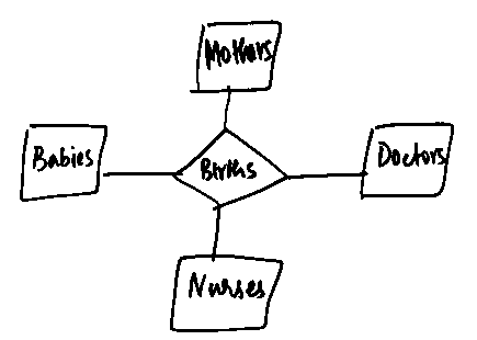
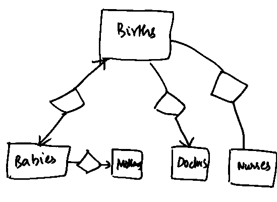
- The answer to part (4) is given below. Notice that
now births takes on an "existence" of its own; it thus has to
become an entity set; we can easily do it by "pushing-out"
and then enforcing the additional constraints given in the question.
If you made "Births" to be a weak-set, you will not lose points.
But make sure, that the key(s) for Births are consistent with the
constraints given in the question.
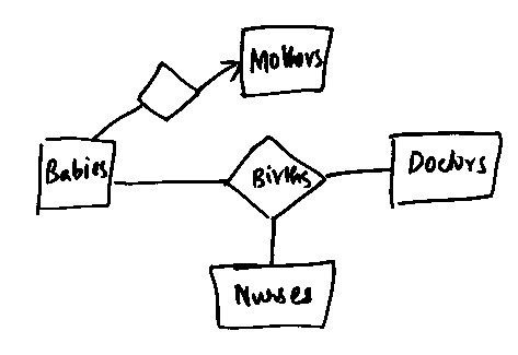
- Similarly for the last part. Notice that all we do here
compared to the previous part is to remove some potential arrows.
A first attempt results in:
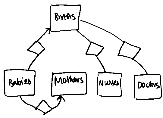 However, this diagram allows tuples of the form:
Birth1  Baby1  Mother1
Birth1  Baby2  Mother1
Birth2  Baby3  Mother2
Birth1  Baby4  Mother3
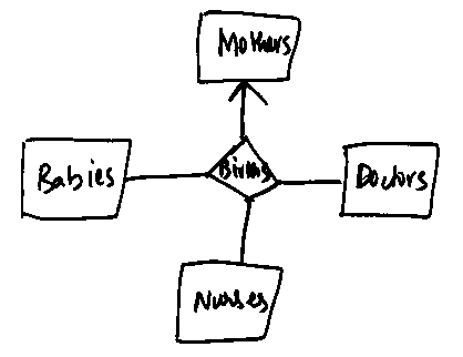
Notice the last tuple which shows that a Birth can involve more than one Mother. This is obviously not what the question intends - a common sense judgement-call (Courtesy Batul Mirza). One attempt at revision would be to introduce a many-one relationship from Births to Mothers, like so: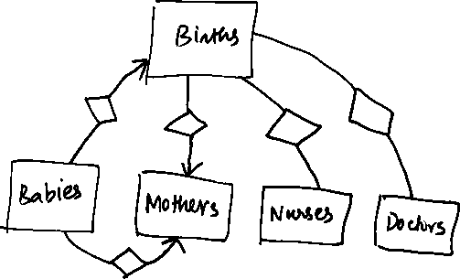 However, this causes redundancy. We thus remove the many-one from Babies
to Mothers (since we can get to a mother anyway through the Birth set).
Notice that a many-one relationship from A to B and a many-one from
B to C implies a many-one from A to C.
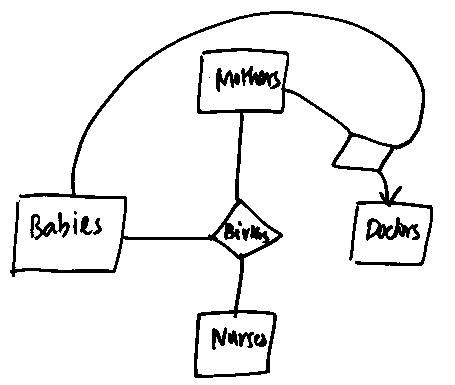
The final diagram thus becomes:
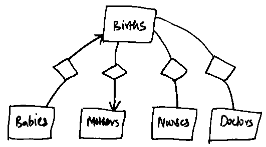
However, this causes redundancy. We thus remove the many-one from Babies
to Mothers (since we can get to a mother anyway through the Birth set).
Notice that a many-one relationship from A to B and a many-one from
B to C implies a many-one from A to C.
The final diagram thus becomes:
Algorithm Naive-Closure
Answer = {X}
Do
   Foreach FD A->B in the given set
	If A is a subset of Answer, then Answer = Answer U B
Until Answer doesn't change (how would you determine this?)
It is easy to see that you might need to do two complete "sweeps" in the worst-case, leading to a quadratic time algorithm. The intuition behind the linear time algorithm is as follows: You take some extra space to "preprocess" the given set of FDs so that each FD gets "fired" at exactly the right moment when you have all the attributes on the left hand side of it. To do this efficiently, you need to first precompute two functions, one from attributes to the FDs they can help "fire" and another from FDs to the number of attributes that are needed to "fire" them (a running counter). This is to save us a lot of overhead in book-keeping. We present these in a pseudo-C fashion:
- FD* atof( ATTR a) is a function that takes an attribute "a" as input
and spits out a list of FDs for which "a" appears on the left hand side.
Notice that this function can be "designed" in O(nm) time, where "n"
is the number of FDs and "m" is the number of attributes. How?
- int ftoa[FD f] is an array (a function in the
mathematical sense) indexed by FDs (like an FD-id). In other words,
it takes an FD as input and returns the number of attributes on the
left hand side of the FD. This function can be "designed" in O(n) time.
Initially this array will contain the full number of attributes
needed to fire, which we will decrement as we keep adding attributes
to our closure. Neat!
Answer = {};
Algorithm Closure
Foreach attribute "a" in X
	Answer = Answer U {a};
	Foreach FD f in atof(a)
		ftoa[f] = ftoa[f] - 1; /* why? */
	        /* check if it is ready to fire */
		if (ftoa[f] == 0) {
			Closure(Y) where Y is the right hand side of FD f;
		}
Why does this work? If you traverse it carefully, you will see that this algorithm is being really selective in the order of FDs that it fires and how it adds attributes. Moreover, once fired, an FD is never used again. It is thus linear in the size of the FDs (which is the sum total of the attributes in each of the FDs). We leave this proof to the reader (it is a simple complexity analysis of a recurrence equation). Also notice the tail-recursive nature of the algorithm; the recursion can be elegantly removed if this is an issue.